-
Inserting and Deleting Columns and Rows
Managing your data often means adjusting your worksheet layout. Whether you’re adding new data fields or removing unnecessary ones, knowing how to insert and delete multiple columns efficiently can save you time and keep your spreadsheet organised.

Watch: How to insert or delete rows and columns in Microsoft Excel
Watch the video below for a quick demonstration on how to add and delete columns and rows.
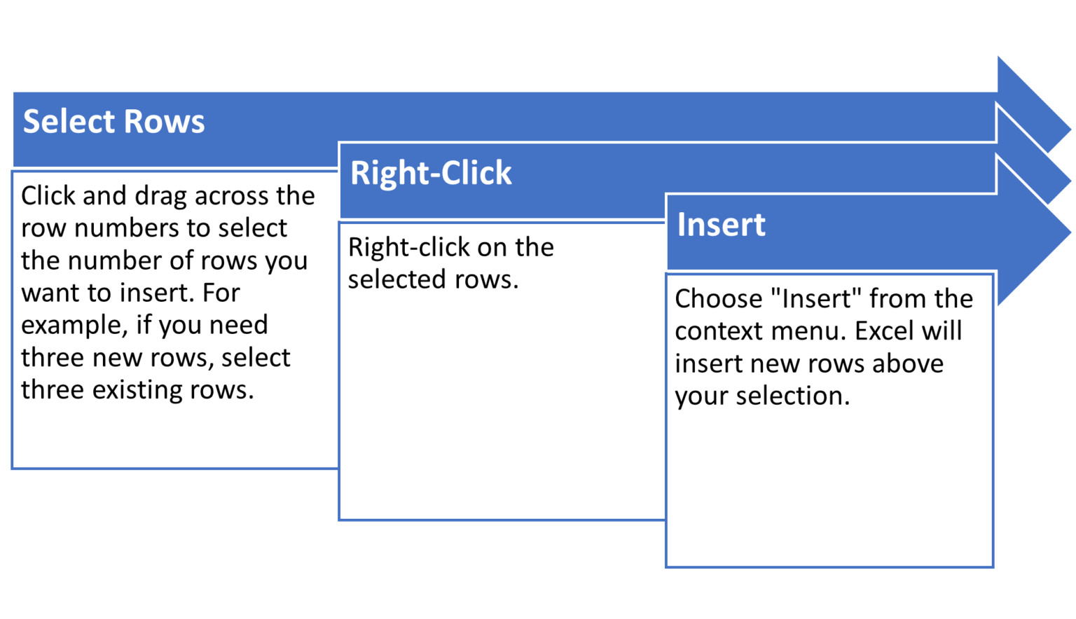
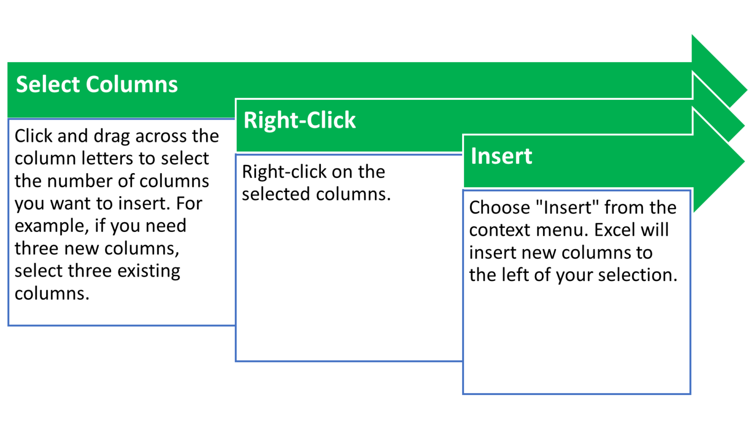
Inserting Columns and Rows
Need more space? Here’s how to add multiple columns or rows at once:
Deleting Columns and Rows
Equally, clearing out unnecessary columns and rows can help declutter your worksheet:
Columns:
- Select Columns: Click and drag across the column letters to select the columns you want to delete.
- Right-Click: Right-click on the selected columns.
- Delete: Choose “Delete” from the context menu. The selected columns will be removed, and any data within them will be lost.
Rows:
- Select Rows: Click and drag across the row numbers to select the rows you want to delete.
- Right-Click: Right-click on the selected rows.
- Delete: Choose “Delete” from the context menu. The selected rows will be removed, and any data within them will be lost.
-
Aligning Cells
Formatting cells is like adding finishing touches to a masterpiece. It makes your data not only look good, but also easier to understand and interpret. Let’s explore how to perfect your cells and ranges with some essential formatting techniques:
Merge and Unmerge Cells
Watch: How to merge and unmerge cells in Microsoft Excel
Combining cells can be useful for creating headers or grouping related data. Watch the video below for a demonstration.
- Merge Cells: Select the cells you want to combine, then go to the Home tab. In the Alignment group, click “Merge & Centre”. You can also choose “Merge Across” or “Merge Cells” depending on your needs.
- Unmerge Cells: Select the merged cell, then click “Merge & Centre” again to unmerge.
Change cell alignment, orientation and indentation
Proper alignment and orientation improve readability!
- Alignment: In the Home tab, use the Alignment group to adjust text alignment (left, centre, right, top, middle, bottom).
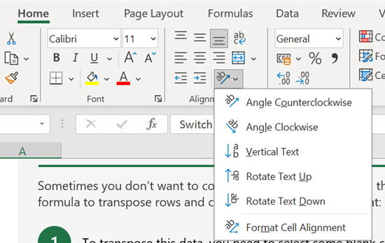
- Orientation: Click the Orientation button to rotate text vertically, diagonally, or at a custom angle.
- Indentation: Use the Increase Indent and Decrease Indent buttons to adjust the indentation of your text.
-
Formatting Cells
Sometimes, your data can be a bit stubborn and refuse to fit nicely in a single cell. Don’t worry! Excel has a magical trick called “Wrap Text” that allows your text to spill into multiple lines within the same cell. It’s like giving your data a cosy blanket!
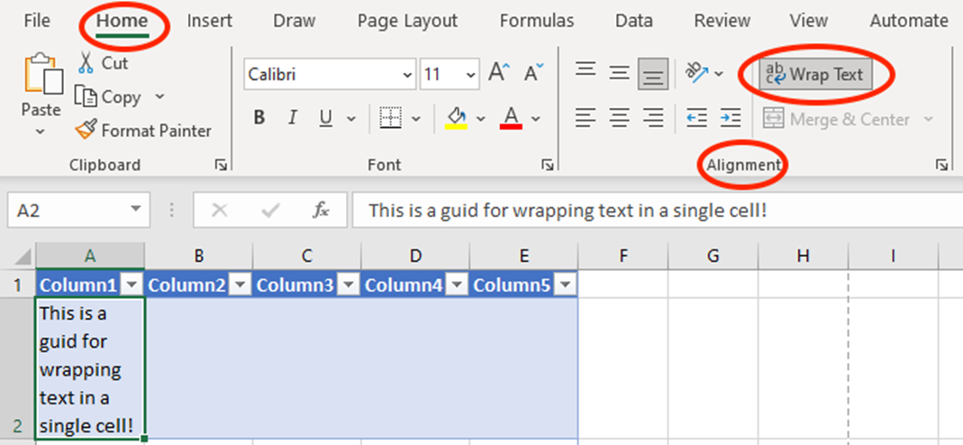
Voila! Your text will now appear neatly wrapped, making your spreadsheet look cleaner and more organised. No more awkward cut-offs or scrolling through long lines of text!
Apply Number Formats
Numbers can wear many hats, and Excel lets you dress them up in a variety of formats. Whether you’re working with currency, percentages, or plain old numbers, applying number formats helps convey the right message.
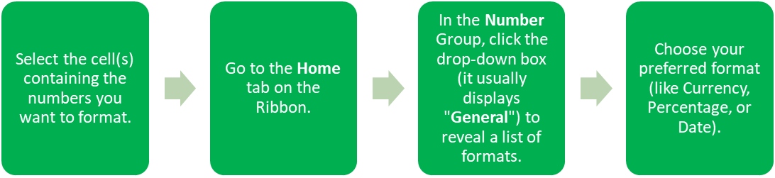
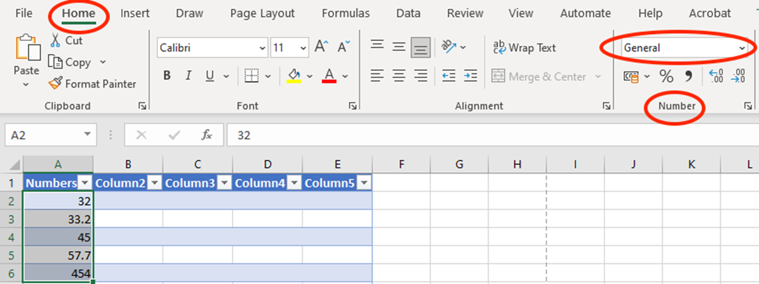
If you’re working with currency, you might want to specify which type of currency to display (like USD, EUR, etc.). To do this, simply:
- Click on “More Number Formats” at the bottom of the drop-down list.
- In the Format Cells window, choose “Currency” or any other format you desire and set your specific options.
By applying number formats, your data will not only look better but also be easier to understand at a glance—no more guessing what those numbers mean!
Apply Cell Styles
Why settle for plain when you can have style? Cell Styles in Excel allow you to jazz up your spreadsheet quickly and easily by adding colours, borders, shading etc.
Think of it as dressing your data in its best outfit—these styles can help highlight important information and make your worksheet visually appealing. University and work assignments will also often require you to apply specific styles to your spreadsheet – so this is a useful thing to know!

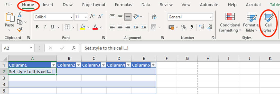
With just a few clicks, your data will be looking sharp and ready to impress!
Clear Cell Formatting
Sometimes, you might want to strip your cells of all those fancy styles and formats to start fresh. Think of it as giving your data a clean slate.
How to Clear Cell Formatting:
- Select the cell(s) from which you want to remove formatting.
- Head to the Home tab on the Ribbon.
- In the Editing Group, click on the “Clear” drop-down arrow.
- Choose “Clear Formats.”
And just like that, your cells will revert to their default formatting, ready for new styles or formats.
-
Try it Yourself
Well done!
You are doing a brilliant job completing the second section of this Self Study Pack.
Now it’s time for more practice . . .
We will be using the same dataset in this section. You can either continue completing the next set of tasks in the same file you used in the previous section, or download the new file below.
Download: 2. Manage Data Cells and Ranges

Apply Your Thinking
Complete the below list of tasks to improve your skills in managing data cells and ranges.
- Import the spotify_songs.csv file into the “SpotifyData” worksheet using the “Data” tab. Before proceeding with this task, you need to either make sure you have downloaded the csv file in the green box below, or open the file you used in the previous section.
- Insert two new columns to the left of the “artist” column in the “SpotifyData” worksheet. Label these new columns “Album” and “Release Date”.
- Delete the “popularity” column from the “SpotifyData” worksheet.
- Insert a new row above the header row (row 2). In the new row, add the title “Top Spotify Songs” across cells A1 to H1.
- Delete rows 10 to 12 from the “SpotifyData” worksheet.
- Merge cells A1 to G1 and Merge & Center the text “This table contains the content of your Spotify dataset:” in the “SpotifyData” worksheet.
- Change the cell style of the header row (row 2) of your Spotify Songs table to “Light Green, 40% – Accent3”.
- Select the “duration_ms” column and format the cells to use thousand separators, ensuring that no decimal points are displayed.
- Apply a conditional formatting rule to highlight songs with a tempo greater than 140 BPM in the “tempo” column.
- Use the “Number Format” option to format the “year” column to show only the last two digits.
- Sort the dataset by “year” in ascending order.
- Filter the dataset to show only the “rock” genre songs.
- Filter the dataset to display songs with a popularity score greater than 70.
If you struggle with any of these tasks – don’t worry! You can view the solutions in the file below.
