Calculate and Transform Data

Perform Operations by Using Formulas and Functions

Activating Excel Functions

Before we dig into the details of calculating and transforming data, let’s clarify how to activate Excel functions:

Important!

To use any function in Excel, you need to start by typing the equals sign (=) on your keyboard. This tells Excel that you’re about to perform a calculation or operation.

In this next section, we’ll explore how to perform various calculations and transformations using Excel’s powerful functions. Remember, you don’t always have to type out cell ranges manually! You can simply select the cells you want after calling out the function. Let’s go!

Calculation Functions

AVERAGE(), MAX(), MIN() and SUM()

Excel is equipped with a suite of functions that can help you quickly calculate essential metrics.

• AVERAGE(): Calculates the mean value of a range of numbers.
• MAX(): Finds the highest value in a range.
• MIN(): Finds the lowest value in a range.
• SUM(): Adds up all the numbers in a range.

Here’s how to use some of the most common functions:

How to Use These Functions:

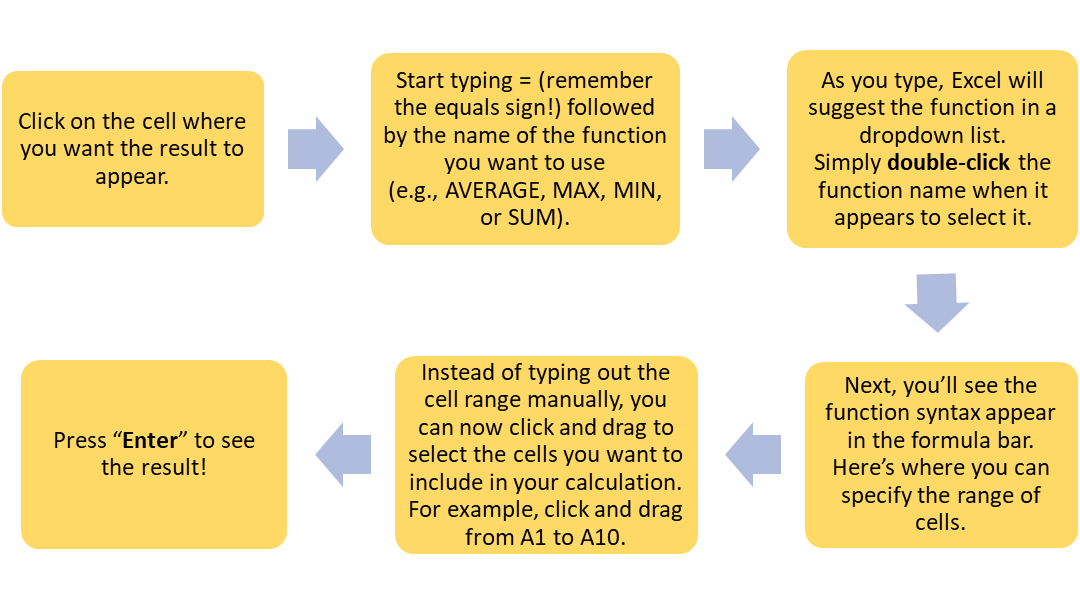
These functions are fundamental for any data analysis, allowing you to quickly summarise and understand your data.

Counting Functions: COUNT(), COUNTA() AND COUNTBLANK()

Counting cells is crucial for data analysis, especially when you need to know how many entries you have. 

Watch: Using Count and CountA in Excel

Watch the below video to learn a bit more about these functions.

Here’s what these functions do:

• COUNT(): Counts the number of cells that contain numbers in a range.
• COUNTA(): Counts the number of non-empty cells in a range, regardless of the type of data.
• COUNTBLANK(): Counts the number of empty cells in a range.

How to Use These Functions:

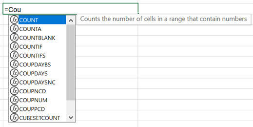
1. Click on the cell where you want the count to show.
2. Start typing = followed by the function you need (e.g., COUNTA).
3. As you type, the function will appear in a dropdown list. Double-click the function name to select it.
4. The syntax will appear for you to fill in the range. Instead of typing, click and drag to select the cells you want to count.
5. Hit “Enter” to display the count.

These counting functions help you keep track of your data entries, ensuring you always know how many records you’re working with.

Conditional Operations: If() Function

The IF() function allows you to execute conditional logic in your spreadsheets—think of it as a “choose your own adventure” for your data. You can perform different calculations based on whether a condition is met or not.

How to Use the IF() Function:

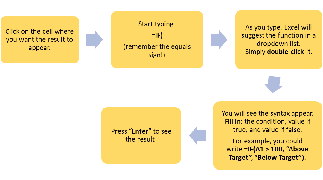
With the IF() function, you can create dynamic analyses that adjust based on your data.

Watch: How to use the IF function in Excel

It seems a bit complicated right? Do you still confused on how to use the IF function? Watch the video below for a demonstration.

Sorting Functions

SORT()

The SORT() function allows you to dynamically sort data in a specified order. This is especially useful when you want to create a sorted list without altering your original data.

How to Use the SORT() Function:

1. Click on the cell where you want the sorted data to appear.
2. Start typing = followed by SORT(. As you type, the function will show up in the dropdown list.
3. Double-click the SORT function to select it.
4. Enter the necessary parameters such as the array and sort order. You can specify the range as you did before—click and drag to select it.
5. Hit “Enter” to display the sorted data.

With the SORT() function, you can easily keep your data organised and accessible!

Watch: Sorting in Excel – Basics and Beyond

Do you want to learn a bit more about how to sort information in Excel? Watch the below video to see some demonstrations.

UNIQUE()

The UNIQUE() function is a fantastic tool that helps you extract distinct values from a range.

How to Use the UNIQUE() Function:

1. Click on the cell where you want the unique values to show.
2. Start typing = followed by UNIQUE(. The function will pop up in the dropdown list.
3. Double-click the UNIQUE function to select it.
4. Enter the range by clicking and dragging over the cells you want to include.
5. Press “Enter” to see the list of unique values.

This function is a real time-saver when you want to analyse data without the clutter of duplicates!

Formatting Text Functions

Text manipulation is essential for presenting your data clearly and effectively. Whether you need to extract specific words, or change your text to upper or lower case letters, Excel offers powerful functions to help you. 

Note

As always, remember to activate any function by starting with the equal sign (=) on your keyboard.

Let’s get started!

Using RIGHT(), LEFT(), and MID() functions

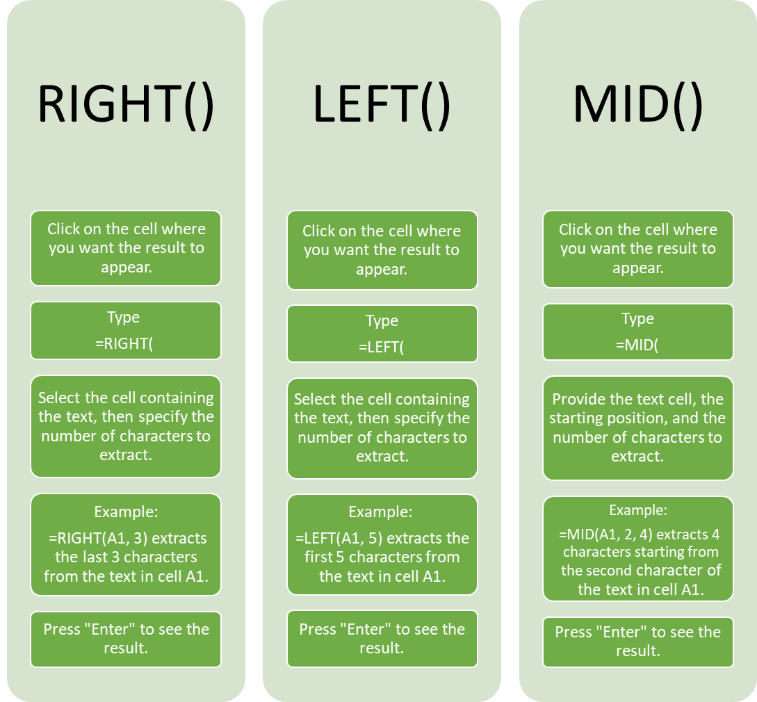
Need to extract specific parts of text? Excel’s RIGHT(), LEFT(), and MID() functions are here to assist!

• RIGHT(): Extracts a specified number of characters from the end of a text string.
• LEFT(): Extracts a specified number of characters from the start of a text string.
• MID(): Extracts characters from the middle of a text string, based on a starting position.

The steps to use each of these functions have been included in a handy image below:

Using UPPER(), LOWER(), and LEN() functions

Want to change the case of your text or find out how long it is? Excel has you covered with UPPER(), LOWER(), and LEN() functions!

• UPPER(): Converts all characters in a text string to uppercase.
• LOWER(): Converts all characters in a text string to lowercase.
• LEN(): Returns the number of characters in a text string.

How to Use These Functions:

1. UPPER():
   • Click on the cell where you want the uppercase text to appear.
   • Type =UPPER( and double-click the function name when it appears.
   • Select the cell containing the text you want to convert.
   • Press “Enter” to see the result.

Example: =UPPER(A1) will convert the text in cell A1 to uppercase.

1. LOWER():
   • Click on the cell where you want the lowercase text to appear.
   • Type =LOWER( and double-click the function name when it appears.
   • Select the cell with the text you want to convert.
   • Press “Enter” to see the result.

Example: =LOWER(A1) will convert the text in cell A1 to lowercase.

1. LEN():
   • Click on the cell where you want the length to show.
   • Type =LEN( and double-click the function name when it appears.
   • Select the cell containing the text you want to measure.
   • Press “Enter” to see the result.

Example: =LEN(A1) will reveal the number of characters in the text in cell A1.

Using the CONCAT() and TEXTJOIN() functions

When it comes to combining text, CONCAT() and TEXTJOIN() are your best friends!

• CONCAT(): Combines multiple text strings into one.
• TEXTJOIN(): Combines multiple text strings with a specified delimiter (like a comma or space) and can ignore empty cells.

Hold on – what is a string?

Note

In Excel, blocks of text that appear in your spreadsheet are often called strings. This can include anything from names, to email addresses, to product descriptions. When you enter text directly into a cell, Excel will automatically treat it as a string.

How to Use These Functions:

1. CONCAT():
   • Click on the cell where you want the combined text to appear.
   • Type =CONCAT( 
   • Double-click the function name.
   • Select the cells you want to combine.
   • Press “Enter” to see the result.

Example: =CONCAT(A1, ” “, B1) combines the text from cells A1 and B1 with a space in between.

1. TEXTJOIN():
   • Click on the cell where you want the combined text to appear.
   • Type =TEXTJOIN( and double-click the function name.
   • Specify the delimiter (e.g., “, ” to separate items with a comma and a space), whether to ignore empty cells, and the range of cells to combine.
   • Press “Enter” to see the result.

Example: =TEXTJOIN(“, “, TRUE, A1:A5) combines the text from cells A1 to A5, separated by commas, while ignoring any empty cells.

Stop and Reflect

Before you move on, take a moment to pause and reflect on the significance of this section. 

The skills you’ve just learned—calculating, transforming data, and formatting text—are not only foundational to mastering Excel, but also frequently tested in exams.

Try it Yourself

Pay Close Attention!

Make sure to practice these functions extensively. The more comfortable you become using the functions we covered, the better prepared you’ll be for any exam or workplace scenario. Set aside time to work through examples and challenges to solidify your understanding.

Remember, practice makes perfect, and this section is a treasure trove of knowledge that will serve you well beyond this course. Happy practicing!

Below is the file you will be working with to finish this section.

Download: Formulas and Functions

Apply Your Thinking

Download the file above and complete the following tasks to practice your skills using formulas and functions.

1. In cell G2, insert a new table heading titled ‘Balance’.
2. Add a thick, black border around cells B2:G25.
3. In column G, calculate the total balance after each transaction.
4. Generate a cell rule that highlights any balance less than zero using ‘light red fill with dark red text’.
5. For added detail, try and create your own conditional formatting rule using some of the other options available.
6. Find the AVERAGE grocery expense, input this into cell D22.
7. Find the AVERAGE Utilities expense, input the result into D23.
8. Find the AVERAGE Rent expense, input the result into D24.
9. Find the MAX expense in January, input this into cell D25.